filtering updates on lie groups

moving gaussians around curves

$\require{boldsymbol}$ Robot navigation is the task of determining a robot state from noisy sensor measurements, and therefore involves statistics and errors. However, our robot states often involve rotations, which raises questions on how we add and subtract rotations. We have to reconsider addition, subtraction, integration, and so on. We need Lie groups (some notes on Lie groups, and they are also covered in and ).

In this post I specifically focus on how we move gaussians around on Lie groups. Our robot belief is typically a gaussian. In cases where there are no rotations, and our robot state lives in a vectorspace where everything is nice. The robot state $\mathbf{x}$ is updated, typically through a Kalman filter correction step where the belief is conditioned on a received measurement ( see for detailed expressions ). The initial robot belief is a gaussian $\mathcal{N}(\mathbf{0}, \check{\mathbf{P}})$, that is then updated to $\mathcal{N}(\hat{\mathbf{x}}, \hat{\mathbf{P}})$.

The nice vectorspace case.

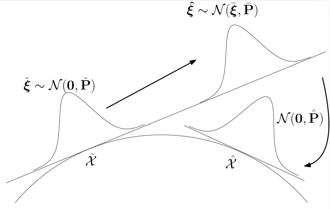
For the Lie group case, the state now lives on a manifold and is denoted $\mathcal{X}$. Notions of addition and subtraction are allowed in the Lie algebra, and in the tangent spaces defined at each $\mathcal{X}$. State beliefs are now represented as concentrated gaussians, where $\mathcal{X}=\bar{\mathcal{X}} \oplus \boldsymbol{\xi}, \quad \boldsymbol{\xi} \sim \mathcal{N}(\mathbf{0}, \mathbf{P})$. The gaussian lives in the tangent space and the distribution over the manifold is defined by its relationship to the tangent space. There are now two steps that must be done to update the robot state. First, in the initial state belief’s tangent space, the gaussian $\check{\boldsymbol{\xi}}$ distributed as $\mathcal{N}(\mathbf{0}, \check{\mathbf{P}})$ is updated to $\mathcal{N}(\bar{\boldsymbol{\xi}}, \bar{\mathbf{P}})$. This is done by writing the measurement model in terms of $\boldsymbol{\xi}$ and carrying out the standard Kalman filter updates on $\boldsymbol{\xi}$. This yields a distribution over $\boldsymbol{\xi}$ with a nonzero mean $\bar{\boldsymbol{\xi}}$. However, when we use concentrated gaussians, we want a distribution of the form $\mathcal{X}=\hat{\mathcal{X}} \oplus \boldsymbol{\xi}, \quad \boldsymbol{\xi} \sim \mathcal{N}(\mathbf{0}, \hat{\mathbf{P}})$, that has a zero mean for $\boldsymbol{\xi}$. We want our robot state belief to be at a given updated state $\hat{\mathcal{X}}$, without any strange tangent space additions.

This whole process is illustrated in the following picture.

The more complicated Lie group case.

The question is then, what are $\hat{\mathcal{X}}$ and $\hat{\mathbf{P}}$? The key point is that the distributions given by $\mathcal{X}=\check{\mathcal{X}}\oplus \hat{\boldsymbol{\xi}}, \quad \hat{\boldsymbol{\xi}}\sim \mathcal{N}(\bar{\boldsymbol{\xi}}, \bar{\mathbf{P}})$ and $\mathcal{X}=\hat{\mathcal{X}}\oplus \boldsymbol{\xi}, \quad \boldsymbol{\xi}\sim \mathcal{N}(\mathbf{0}, \hat{\mathbf{P}})$ are the same distribution, just expressed in different tangent spaces of the manifold.

We can therefore do a bit of math to manipulate $\mathcal{X}=\check{\mathcal{X}}\oplus \hat{\boldsymbol{\xi}}, \quad \hat{\boldsymbol{\xi}}\sim \mathcal{N}(\bar{\boldsymbol{\xi}}, \bar{\mathbf{P}})$.

\begin{align*} \mathcal{X} &= \check{\mathcal{X}} \oplus \check{\boldsymbol{\xi}}, \quad \check{\boldsymbol{\xi}} \sim \mathcal{N}(\bar{\boldsymbol{\xi}}, \bar{\mathbf{P}}) \\ &= \check{\mathcal{X}} \oplus (\bar{\boldsymbol{\xi}} + \tilde{\boldsymbol{\xi}}), \quad \tilde{\boldsymbol{\xi}} \sim \mathcal{N}(0, \bar{\mathbf{P}}) \\ &\approx \left( \check{\mathcal{X}} \oplus \bar{\boldsymbol{\xi}} \right) \oplus \underbrace{ \left. \frac{D(\mathcal{X} \oplus \boldsymbol{\tau})}{D\boldsymbol{\tau}} \right|_{\bar{\boldsymbol{\xi}}} }_{\mathbf{J}_{\tilde{\boldsymbol{\xi}}}} \tilde{\boldsymbol{\xi}}, \quad \tilde{\boldsymbol{\xi}} \sim \mathcal{N}(0, \bar{\mathbf{P}}) \\ &= \hat{\mathcal{X}} \oplus \boldsymbol{\xi}, \quad \boldsymbol{\xi} \sim \mathcal{N}(0, \mathbf{J}_{\tilde{\boldsymbol{\xi}}} \bar{\mathbf{P}} \mathbf{J}_{\tilde{\boldsymbol{\xi}}}^\top) \end{align*}

The crucial step comes in the third line, where we use the Lie group Jacobian of the plus operation, which is the same as the group Jacobian . This Jacobian accounts for the difference in the tangent spaces at $\check{\mathcal{X}}$ and $\hat{\mathcal{X}}$. This explains the presence of the Jacobian in Lie group filter estimation codes such as in our lab’s navlie library. For a small update, where $\tilde{\boldsymbol{\xi}}$ is small, this Jacobian is close to identity. However, for larger updates, neglecting it can cause inaccuracies in the updated covariance $\hat{\mathbf{P}}$.